
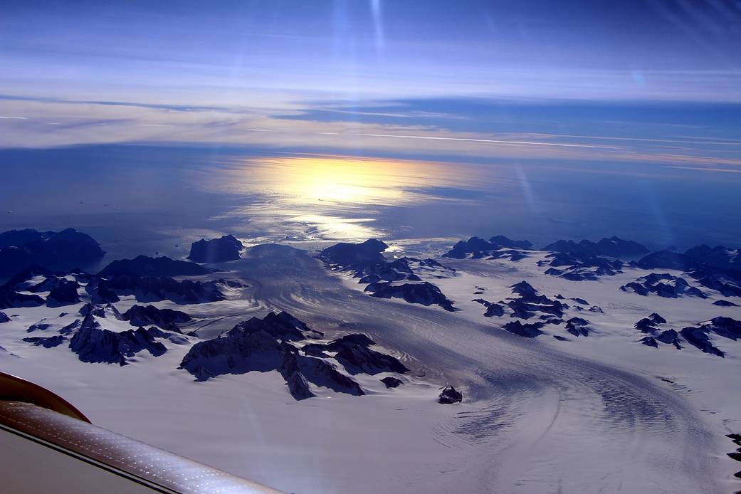
A more connected landscape under the ice
NASA’s September 28 Earth Observatory feature presents research that mapped 1,943 valleys beneath Greenland’s ice sheet, with roughly a third newly identified. The underlying paper, by Allison Chartrand and colleagues in Geophysical Research Letters, was first published on June 30. Today’s feature is a new public explanation of that study, not a new paper released this morning.
The researchers used Ice Flow Perturbation Analysis to infer buried terrain from surface elevation and motion. Their map connects features that earlier representations left fragmented, including valleys extending farther inland. The significance is not an unexplored landscape photographed through kilometres of ice: it is an improved reconstruction from indirect evidence.
For readers interested in technology, this is a useful example of sensing and computation doing different jobs. An instrument measures something accessible; a physical model helps infer something that is difficult to observe directly.
Source notes: 1, 2. Analysis and proposed examples are identified in the text.
What the satellite measures—and what it does not
NASA’s ICESat-2 instrument reference explains that ATLAS times laser photons travelling to Earth and returning to the satellite. Combined with the spacecraft’s position, those measurements help determine surface height. Processing must distinguish the relevant returns from background light and other signals.
That measurement is not, on its own, the depth of a buried valley. Our explanation is to imagine two separate questions: where is the visible surface, and which underlying shape could help produce the observed surface and movement? Answering the second requires more information and assumptions than answering the first.
This separation matters whenever a striking scientific image is described as a “scan.” A coloured reconstruction can be grounded in measurements without every coloured point representing a direct observation of the hidden object. Readers should look for the instrument, the measured quantity and the inference connecting it to the image.
Source notes: 3. Analysis and proposed examples are identified in the text.
An inverse problem, not a tracing exercise
The study describes a method that uses the way variations at the bed affect surface elevation and ice velocity. The authors apply a modified inversion approach and compare the result with observations and BedMachine Greenland. Its purpose includes improving the slow-moving interior, where existing constraints are relatively sparse.
Lumacta’s scientific interpretation is that an inverse problem works backwards from an effect to a possible cause. This is powerful, but a visually plausible answer is not sufficient validation. One must ask whether other combinations of conditions could fit the observations and whether the method performs well where independent measurements exist.
A useful way to evaluate an inferred feature is to check what constrains it locally. Is there a nearby radar measurement, a strong surface signal or mainly a model-based continuation? Those are different strengths of evidence. We have not reprocessed the satellite data or calculated a new uncertainty map.
Source notes: 2. Analysis and proposed examples are identified in the text.
Grid spacing is not the same as certainty
The NSIDC catalogue describes BedMachine Greenland Version 6 as a combination of bed topography, bathymetry, surface elevation and ice thickness. It lists a 150-metre spatial grid and provides a dataset version and citation. These details identify an existing reference product; they do not mean the September feature has already replaced it.
For a reader or developer, the important distinction is between the spacing of stored values and the confidence of each value. A fine grid can contain areas with very different observational support. Adding more pixels does not automatically add more independent measurements.
Our practical advice for anyone building a visualisation is to preserve the dataset version and make clear whether the display shows measurements, an inferred bed or another derived quantity. A smooth, attractive map should not erase the provenance that lets someone understand and challenge it.
Source notes: 4. Analysis and proposed examples are identified in the text.
Better terrain is an input, not a complete sea-level forecast
The research connects valley geometry to questions about ice flow, drainage and Greenland’s earlier landscape. The paper’s interpretations about geological inheritance and groundwater influence are scientific explanations to investigate, not direct observations of ancient events.
Our interpretation of the climate relevance is deliberately bounded. Changing the terrain input can change what an ice-flow model calculates. It does not supply all the other conditions that determine a future outcome, and this article cannot translate the valley count into a number of centimetres of sea-level rise.
The next useful comparison would hold a model’s other assumptions constant and examine what changes when the updated terrain is included. That would isolate one contribution. It would still need uncertainty estimates and testing against observations before supporting a confident forecast.
Source notes: 1, 2. Analysis and proposed examples are identified in the text.
The achievement is making a hidden boundary more testable
A good scientific map is more than a compelling picture. It makes a claim about the world in a form that can be compared with new observations. In this case, inferred connections between valleys can help focus questions for later surveying and modelling.
Lumacta would judge the advance by how well those connections survive independent checks, not merely by the number of features drawn. Agreement would strengthen the reconstruction; disagreement could reveal where the method or its inputs need improvement. Both outcomes would be scientifically useful.
The takeaway is that satellites need not directly image a hidden surface to help map it. But the inference is part of the result, not a detail to hide. Understanding that distinction makes this a more interesting technology story—and a more honest one.
Source notes: 2, 3, 4. Analysis and proposed examples are identified in the text.
Sources & Methods
Prepared September 28, 2026. We read NASA’s current feature, the June 30 study’s abstract and relevant methods, the BedMachine Version 6 catalogue and ICESat-2 instrument documentation. The inverse-problem explanation and proposed model comparison are Lumacta analysis. No fieldwork, dataset reprocessing, interview or new climate projection was performed.
- NASA Earth Observatory: valleys hidden below Greenland’s ice — September 28, 2026 feature and visual explanation of earlier research
- Chartrand et al.: A Vast Valley Network Beneath the Greenland Ice Sheet — Peer-reviewed paper first published June 30, 2026; methods and interpretation, not independently replicated here
- NASA ICESat-2: Space Lasers — Primary ATLAS instrument explanation, photon timing and surface-height processing
- NSIDC: IceBridge BedMachine Greenland, Version 6 — Reference-product catalogue, grid spacing, version and data provenance